
GEOG 6160 Spatial Modeling and Geocomputation
Using Machine Learning for Alpine Land Classification in Mountainous Terrain
Background & Introduction
Alpine terrain is a crucial research area for scientists across multiple disciplines, including botanists at the Betty Ford Alpine Gardens in Vail, Colorado. While mountains are intuitively recognizable to humans, providing definitive scientific classifications of alpine terrain remains challenging. A rough definition of alpine areas can be described as mountain regions where a combination of temperature, growing season, elevation, and latitude create conditions unsuitable for tree growth.

Figure 1: Columbine (Aquilegia). Source: Todd Pierce, Betty Ford Alpine Gardens
The Betty Ford Alpine Gardens, dedicated to conservation and education about alpine flora, employs botanists and biologists who conduct field research searching for different alpine plant species (Figure 1). Their work is challenging due to short alpine summers (when snow has melted) and vast alpine areas to explore. This project aims to apply modern machine learning methods to help identify alpine regions more precisely, supporting researchers in focusing their field efforts more effectively.
The Global Mountain Biodiversity Assessment (GMBA) has adopted the concept of "ruggedness" to define mountains, focusing on local elevation changes rather than absolute elevation. Additionally, Testolin et al. (2020) developed a comprehensive global map of alpine areas using 19 climatic variables, though some regions like the Tarryall Mountains (Figure 2) in Colorado remain unclassified in their approach.
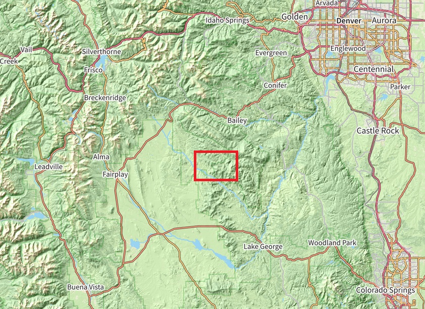
Figure 2: The location of the Tarryall Mountains is denoted by the red box. Source: OpenStreetMap
Machine learning has proven effective for land use land cover (LULC) classification, particularly when combining methods like random forest, support vector machine, and artificial neural networks with satellite imagery. This study explores whether these techniques can be applied successfully to the specific challenge of alpine terrain classification.
Methodology
This study builds upon work by Emily Griffoul (Conservation Scientist at Betty Ford Alpine Gardens) and Dara Seidl (Associate Professor of GIS at Colorado Mountain College). While Griffoul attempted to combine in situ observations with the GMBA mountain inventory using ESRI ArcGIS Pro, the results were not sufficiently accurate and were time-intensive. Seidl achieved better results using remote sensing, digital elevation models (DEMs), and Google Earth Engine (GEE), but encountered limitations in GEE's methodological options.
| Band | Description |
|---|---|
| 1 | Visible Coastal Aerosol (0.43 - 0.45 μm) |
| 2 | Visible Blue (0.450 - 0.51 μm) |
| 3 | Visible Green (0.53 - 0.59 μm) |
| 4 | Red (0.64 - 0.67 μm) |
| 5 | Near-Infrared (0.85 - 0.88 μm) |
| 6 | SWIR 1(1.57 - 1.65 μm) |
| 7 | SWIR 2 (2.11 - 2.29 μm) |
Figure 3: Landsat 9 OLI-2 Bands. Source: USGS
This study employed similar techniques to Seidl's but utilized random forests and neural networks in R. Landsat 9 OLI-2 imagery (Figure 3) was collected for summer months (mid-July to mid-September, 2018 to 2024) to minimize snow effects on reflectance. Cloud coverage was limited to 4% in the data sourced from the USGS, which also provided the DEMs.
Three diverse study areas were selected:
- Parts of the Canadian Rockies, Calgary, Alberta, and southern plains
- Denver, Colorado area, surrounding cities, and mountain ranges in the Colorado Rockies
- White Mountains in New Hampshire and southwestern Maine
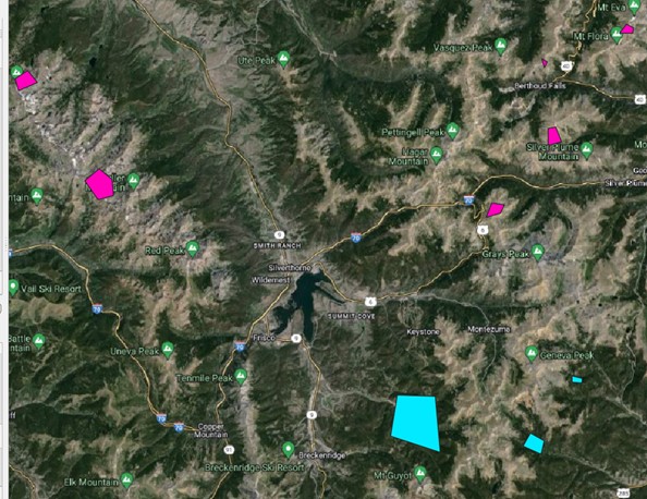
Figure 4: A QGIS screenshot showing a small subset of the polygons used for training data samples. Here, magenta polygons occur in alpine environments, while the cyan ones do not.
Using QGIS, polygons were manually created in each area to represent alpine and non-alpine land cover (Figure 4), resulting in six total shapefiles. These were referenced against Google Maps Satellite imagery. From these polygons, 999 random samples were taken from each shapefile (5,994 points total). Three different raster stacks were created, one for each study area, with eight bands: seven from Landsat 9 OLI-2 and one DEM. All data was scaled to a range of 0-1 based on minimum and maximum values, and N/A values were removed, leaving 5,889 points.
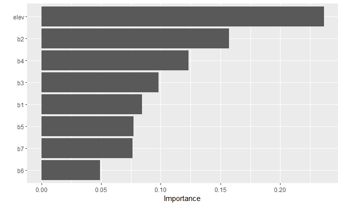
Figure 5: Variable importance plot when all three areas are used, and elevation is included.
Four machine learning models were created using the combined data from all three areas:
- Random forest using only the seven Landsat 9 OLI-2 bands
- Random forest including elevation
- Neural network using only the seven Landsat 9 OLI-2 bands
- Neural network including elevation and latitude
The neural network models used the following parameters: size = 25, decay = 1e-5, maxit = 500. All models were resampled with an 80%/20% holdout strategy, and attempts were made to tune hyperparameters, though none improved the AUC scores.
Results
The random forest model using only Landsat 9 OLI-2 bands achieved an AUC score of 0.97. When elevation was added, the AUC improved to 0.998, with elevation showing considerable variable importance (Figure 5).
The neural network models yielded similar results. Using only remote sensing imagery resulted in an AUC of 0.979, while adding latitude and elevation increased the AUC to 0.999.
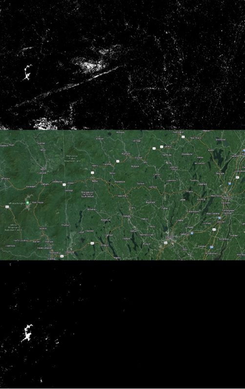
Figure 6: NN Predictions for the White Mountains. Top: Without elevation. Middle: Satellite imagery (source: Google). Bottom: With elevation and latitude
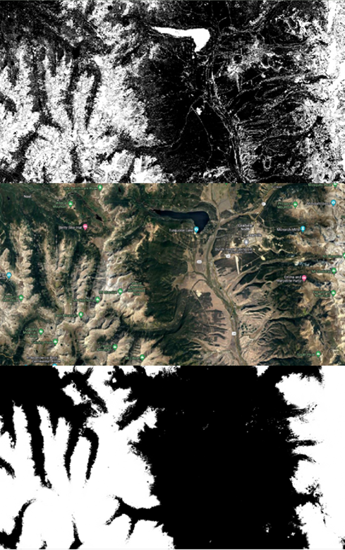
Figure 7: NN Predictions near Leadville, CO. Top: Without elevation. Middle: Satellite imagery (source: Google). Bottom: With elevation and latitude
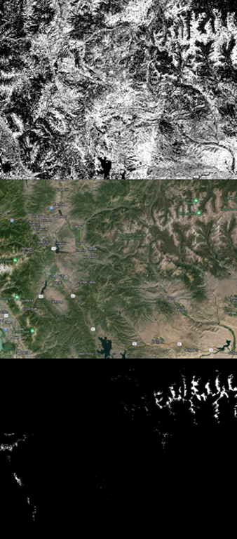
Figure 8: NN Predictions in Utah. Top: Without elevation. Middle: Satellite imagery (source: Google). Bottom: With elevation and latitude
When applied to prediction scenarios (Figures 6, 7, 8), the neural network model using only Landsat 9 OLI-2 bands showed errors of commission. While it captured treeline details effectively, it incorrectly classified pixels below treeline and water bodies as alpine. The model incorporating elevation and latitude created clearer boundaries between alpine and non-alpine regions but had mixed results: it overstated alpine regions in Colorado while understating them in Utah. Neither model correctly classified the Tarryall Mountains as alpine.
Discussion & Conclusion
Despite high AUC scores, the models fell short of producing satisfactory generalized predictions, particularly in Utah (Figure 8). Overfitting appears to be the primary issue, as evidenced by excellent scores but poor performance in new landscapes. This suggests two potential approaches for improvement: using less training data or collecting more diverse training samples from additional landscapes.
The proper treatment of elevation and latitude remains a challenge, as they are strongly associated and can lead to spatial autocorrelation. However, both variables are clearly important in defining alpine regions. Additionally, this work demonstrated the need for significant computational resources when processing and analyzing this type of data, especially when working with neural networks.
This study confirms that machine learning offers powerful tools for land use land cover classification, particularly for alpine environments. While the results did not meet all objectives, they established a promising foundation for future work. Combining spectral data with bioclimatic variables, elevation, and latitude could yield more comprehensive alpine classification systems as computational capabilities advance.
Skills Used
- Machine Learning (Random Forest and Neural Networks)
- Remote Sensing and Image Analysis
- Land Use Land Cover Classification
- R Programming
- QGIS Spatial Analysis
- Digital Elevation Model Processing