
GEOG 5170 Geospatial Field Methods
Data Collection from Bonderman Field Station
Background & Introduction
Cartography has been considered both an art and a science, with debates about whether these are separate concepts. In today's data-driven world, maps serve countless purposes from navigation to locating restaurant reviews, yet it is the artistic elements of cartography that enable clear communication of data for effective use. At Bonderman Field Station at Rio Mesa (Bonderman), students had the opportunity to create maps using various techniques, allowing exploration of the balance between cartographic art and science.
Before creating a map, in situ methodologies can provide crucial data and verification, even when remote collection is possible. Field methods also foster a deeper understanding of the subject matter. This project involved three progressive mapping approaches: first creating hand-drawn maps of selected features at Bonderman, then using ESRI's Field Maps to create digital records, and finally using an unmanned aerial vehicle (UAV) to capture aerial photography for reconstruction.
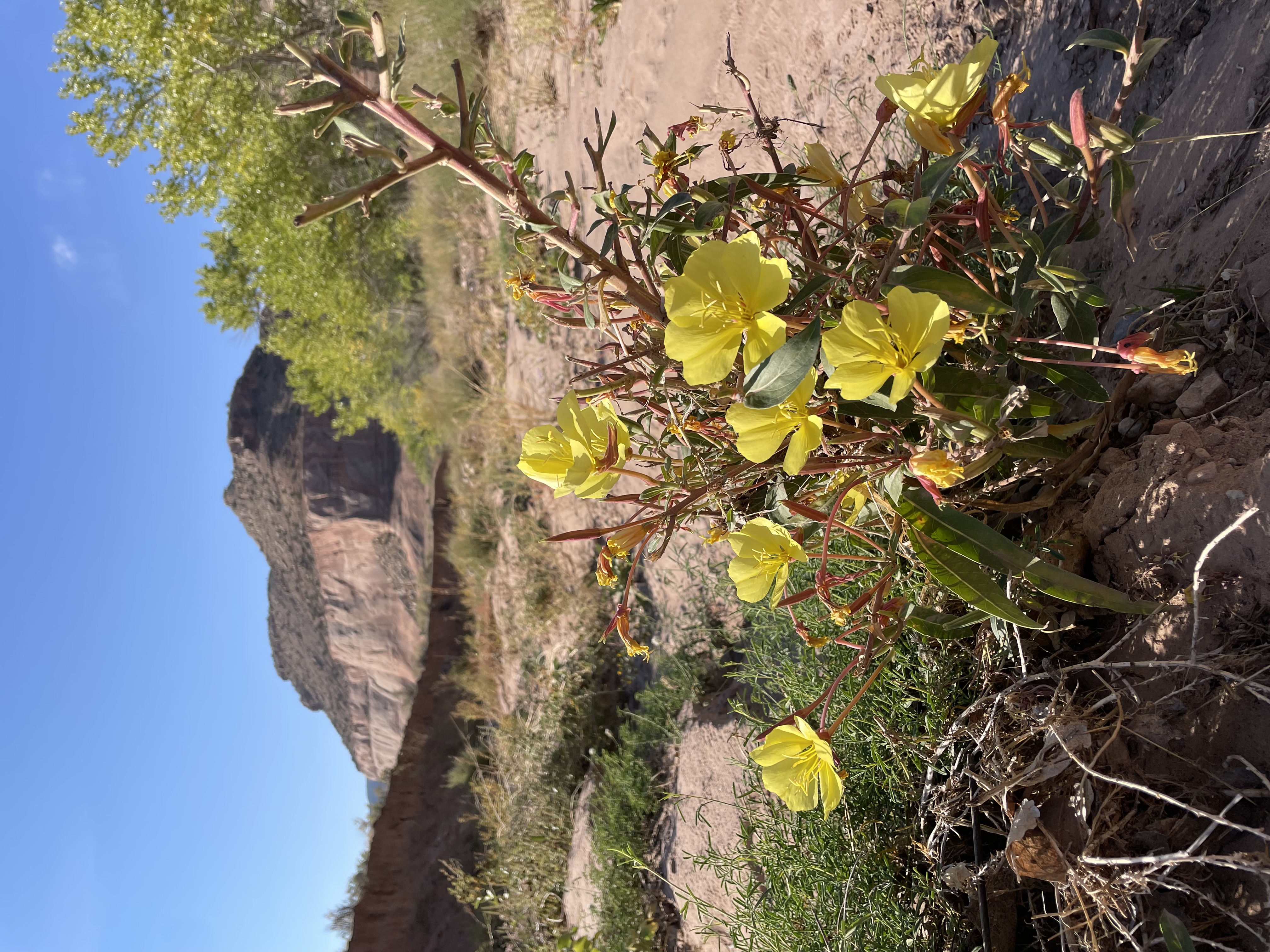
Figure 1: Yellow Evening Primrose at Bonderman Field Station.
Study Areas
Part 1: Culvert Wash Area
The first study area was located approximately 0.8 miles past the Bonderman gate, centered on a concrete culvert where a wash crosses the road. This wash drains northward into the Delores River, supporting vegetation like rabbitbrush and yellow evening primrose (Figure 1). The area also contained manmade features including a weather station and streamgage. The site was selected for its ease of traversal via the wash, nearby roads, and a trail, which allowed observation without disturbing sensitive cryptobiotic crusts.
This north-south oriented study area included the weather station, gaging station, and a USGS Survey marker at the northern end near an access road to the Delores River. A trail to an old icehouse was located at the southern end. The wash contained substantial vegetation, with cottonwoods growing along its edges and evidence of significant flooding visible on the banks. In total, 14 vegetation observations, 10 manmade feature observations, 4 geological observations, and 2 hydrological observations were recorded.
Part 2: Slickrock Bowl and Wash
For the second part of the project, teams selected areas just outside Bonderman. Our team's site was located 2.6 miles from Bonderman, featuring a slickrock bowl with a ridge above it. Between the bowl and road was a wash running southwest to northeast, which contained trees and shrubs. The slickrock bowl displayed geological striations and required careful traversal, while the ridge above offered a panoramic view of the entire study area. The wash area contained diverse flora including trees, shrubs, cacti, and succulents, surrounded by cryptobiotic soil. The terrain provided both dramatic and subtle elevation changes, ideal for testing digital surface model (DSM) accuracies, while remaining safely traversable with good visibility for UAV operations.
Methodology
Part 1: Traditional to Digital Mapping
The initial task involved creating a hand-drawn map using a Rite in the Rain All-Weather Field notebook and pen (Figure 2). The gridded notebook facilitated scale approximation. With the culvert as a center point, the study area was surveyed on foot along the wash, road, and trail, with attention-grabbing features marked on the map. Vegetation was denoted by asterisks, while other features received brief descriptions. North orientation was established with a compass and added to the map. Scale was approximated by counting strides between features, with two short steps estimated as one foot.
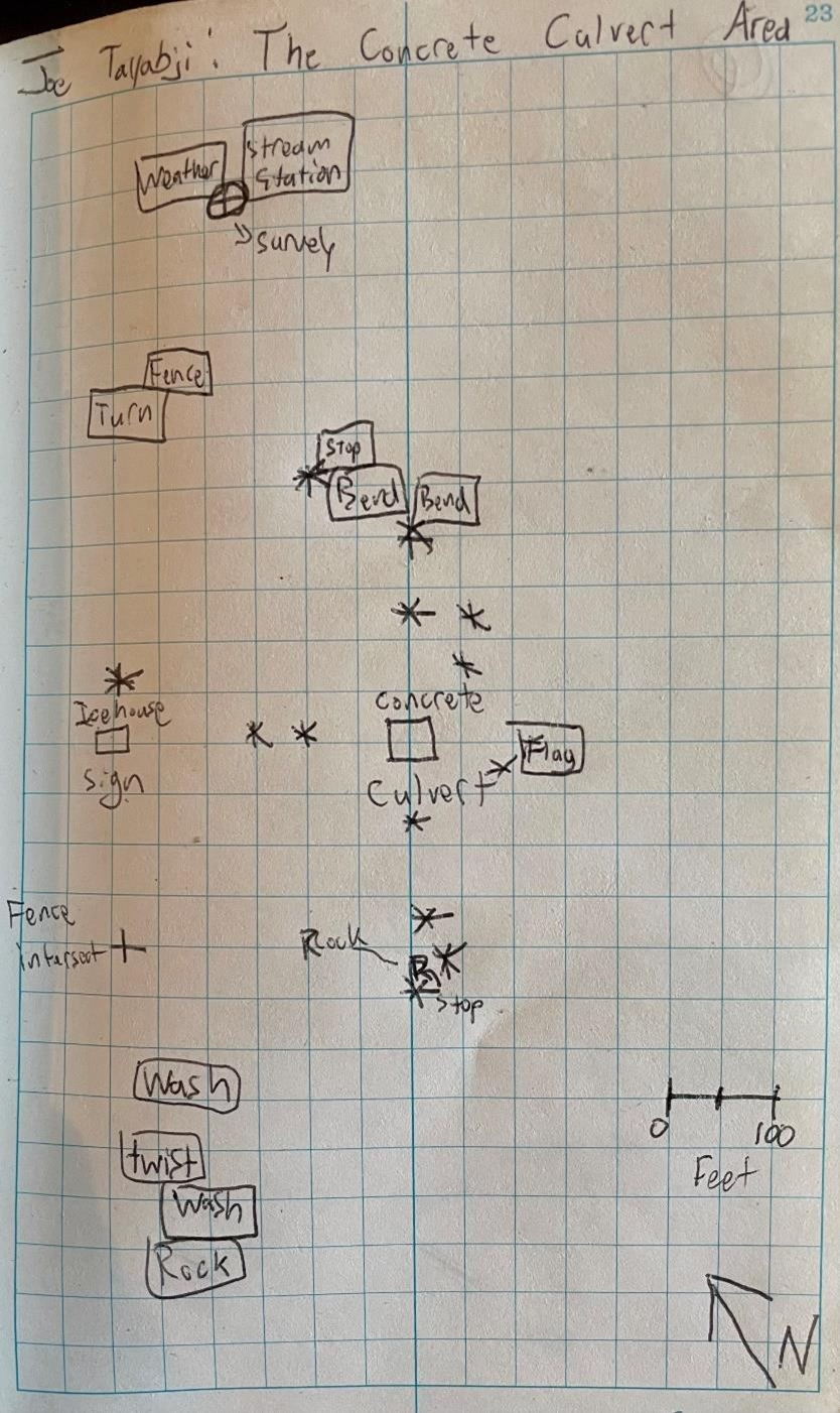
Figure 2: A hand drawn map of the culvert wash area.
Following the hand-drawn mapping, ESRI's Field Maps app was employed using a pre-downloaded section of the Bonderman Field Station map for offline use. The study area was resurveyed with the hand-drawn map as reference. Four feature classes were documented: Built Infrastructure, Hydrology, Biology, and Geology. Each feature received descriptive notes and photographs when possible.
Finally, a DJI Mini drone captured aerial photography after placing 10 ground control points (GCPs) throughout the study area, with locations measured using a high-quality receiver. The UAV flew approximately 30 meters above ground level in a single overlap pattern, with some compromises in flight parameters due to battery concerns. The captured images were processed in Agisoft Metashape Professional, using structure from motion (SfM) techniques to create an orthomosaic. This process involved generating a sparse point cloud, georeferencing images, creating a dense point cloud, building a digital elevation model (DEM), and finally producing the orthomosaic, which was then combined with Field Maps data for the final product (Figure 3).
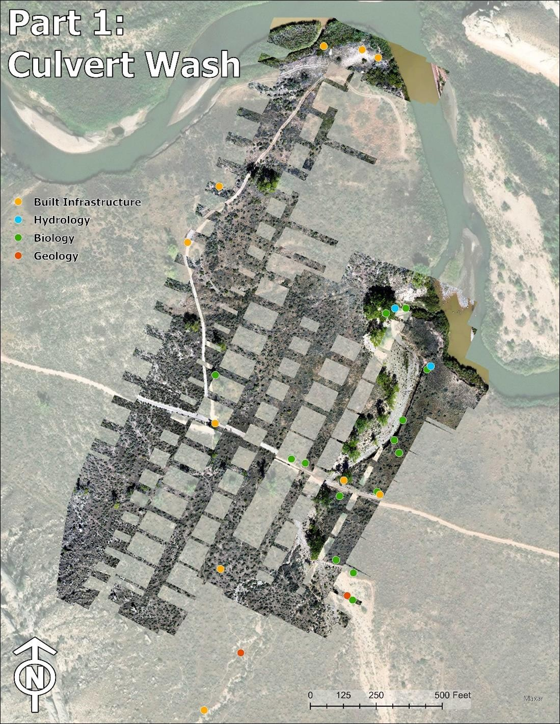
Figure 3: Field Maps data over an incomplete orthomosaic.
Part 2: Advanced Terrain Analysis
The second portion of the project involved comparing different technologies for terrain mapping. Team GCP developed a detailed preflight plan covering flight parameters and ground crew responsibilities. The independent variable tested was the DJI Mini's altitude, with one flight attempting to follow terrain and another maintaining a constant height of 70 meters above takeoff. Ten GCPs were strategically placed throughout the study area (Figure 4).
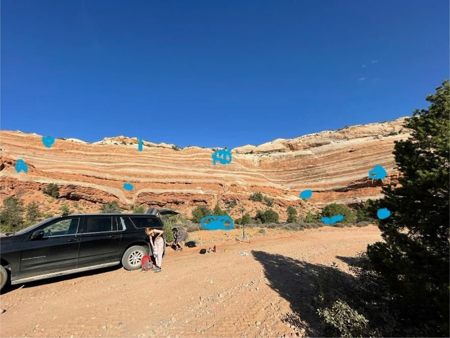
Figure 4: Markup was used on an iPhone photo to determine where the GCPs would be placed before the ground crew split up.
The preflight planning established pilot roles, flight patterns (single overlap), battery management, and communication protocols. Ground crew members placed GCPs at predetermined locations and positioned themselves to maintain visual contact with the UAV throughout operations, with hand signals established to indicate potential hazards. Clear communication procedures were established among all team members as part of the preflight checklist.
After completing the two DJI Mini flights, a LiDAR-equipped UAV was deployed. This involved calibration and setting up a receiver for real-time kinematic (RTK) processing. The LiDAR UAV followed an automated flight plan, collected data, and returned to base upon completion.
The DJI Mini images were sorted by flight using file timestamps and processed in Agisoft Metashape as separate projects. The 70-meter flight captured eight of ten GCPs with an average error of 10.5 meters, while the terrain-following flight captured only four GCPs with an average error of 2.4 meters. For both flights, processing continued with dense point cloud generation, DEM creation, and orthomosaic production. The DEMs and orthomosaics were imported into ArcGIS Pro for analysis.
The LiDAR data was also processed in ArcGIS Pro, creating a 3D scene (Figures 6, 7) to visualize the point cloud and generating a digital surface model. Various visualization techniques were explored to create comparative maps.
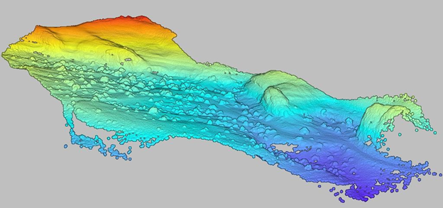
Figure 6: LiDAR point cloud visualized by elevation in ArcGIS Pro.
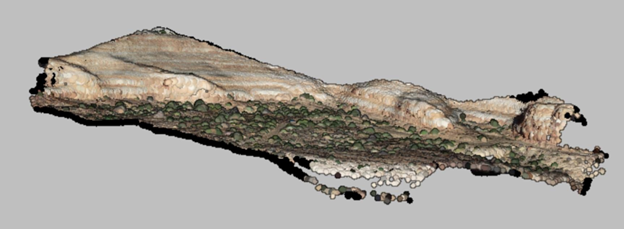
Figure 7: LiDAR point cloud visualized by RGB values in ArcGIS Pro.
Results
Part 1: Traditional vs. Digital Mapping
The hand-drawn map (Figure 2) proved useful for determining relative feature locations despite its limitations. Scale accuracy varied across the map; for example, the distance from culvert to flag appeared as approximately 150 feet on the map and measured 155.7 feet in ArcGIS Pro, while the distance from culvert to northern bend showed greater discrepancy (475 feet on map versus 545.6 feet measured).
The digital map (Figure 3) suffered from missing information in the orthomosaic but offered significantly improved data accuracy from Field Maps despite using consumer hardware. Key advantages included the ability to make precise measurements and endless cartographic adjustments.
Part 2: Terrain Mapping Comparison
Examination of the digital surface models (as hillshades, Figure 8, and aspect-slope visualizations, Figure 9) revealed significant differences in detail and accuracy between methods. The LiDAR data provided exceptional detail, particularly for vegetation, with such fine resolution that individual pixels were distinguishable in the hillshade, creating a textured appearance. Tree canopies were clearly defined.
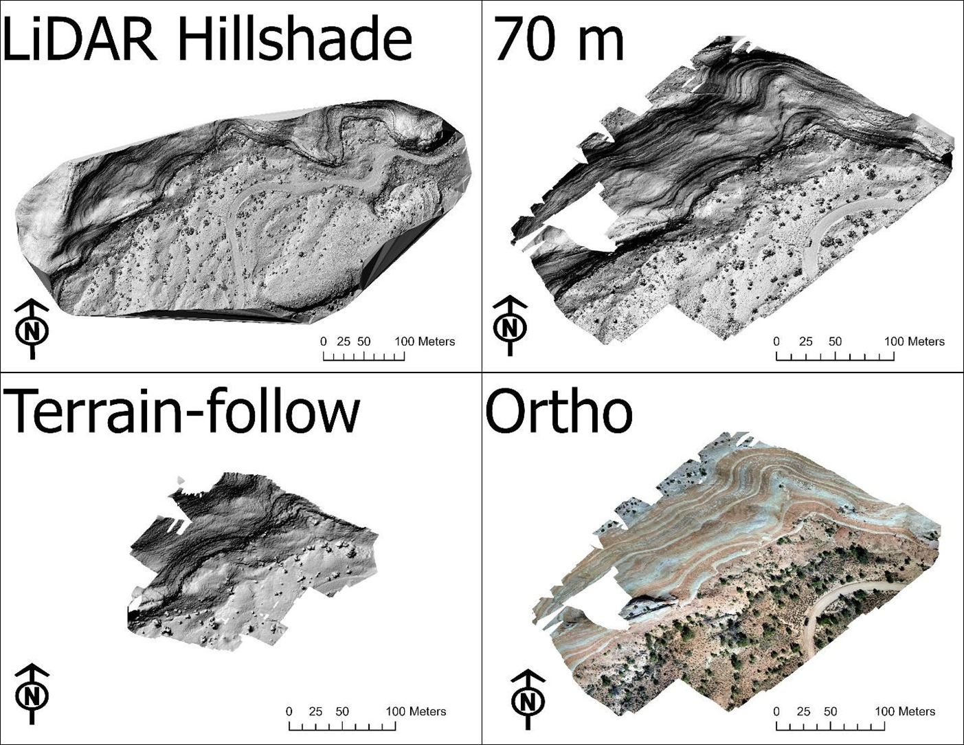
Figure 8: DSMs shown as hillshades.
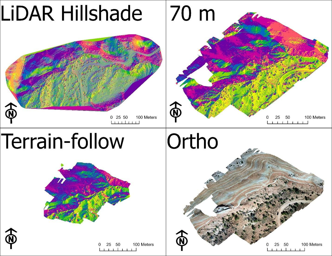
Figure 9: DSMs shown in aspect-slope.
The 70-meter constant altitude flight produced the second-best results, though this may be attributed to capturing more GCPs and achieving finer spatial resolution rather than altitude itself. Vegetation was visible with some detail. The terrain-following flight produced the coarsest data and covered a smaller area, with trees visible but smaller vegetation indistinguishable.
Elevation value differences (Figure 10) between methods appeared related to whether the area was within the bowl formation. The mean difference between LiDAR and the 70-meter flight was -5.3 meters, with values fairly evenly distributed between -20 and 7 meters. Between LiDAR and the terrain-following flight, the mean difference was -13.2 meters with a more bell-shaped distribution. The areas showing positive versus negative differences were essentially inverted when comparing the two differences. Between the two DJI Mini flights, the mean difference was 9.4 meters with a low-side distribution tail.
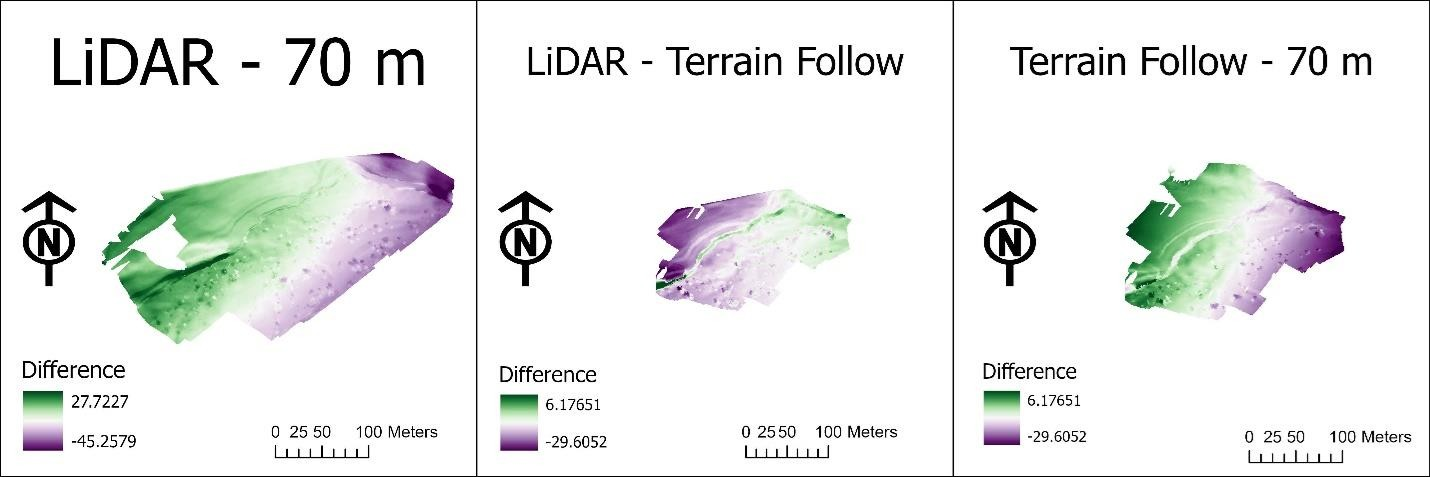
Figure 10: Elevation differences between the different methods.
Discussion & Conclusion
Part 1: Mapping Method Comparisons
Hand-drawn maps retain distinct advantages, including the ability to create them on-site without technology and their usability in adverse weather conditions where electronic devices might fail. However, their accuracy limitations become apparent without technological assistance or significant experience.
Digital mapping techniques offer superior detail and accuracy but require proper planning and technical knowledge. The incomplete orthomosaic resulting from the UAV flight highlighted the importance of proper flight planning and operator experience. Preliminary data downloads, especially in areas without cellular service, are essential for field operations.
Part 2: Terrain Analysis Technology Assessment
The elevation differences between methods appeared strongly correlated with position within the bowl formation, suggesting terrain-following capabilities significantly impact accuracy. The LiDAR data demonstrated superior resolution and accuracy compared to Structure from Motion techniques. However, the critical factor in data quality proved to be the flight execution itself.
The LiDAR UAV, operated by an experienced pilot using automated systems, produced significantly better results than the manually piloted DJI Minis. This underscores the principle that output quality depends fundamentally on input quality—"garbage in, garbage out" applies directly to geographic studies. The analysis can only be as good as the underlying data, emphasizing the importance of careful data collection from the outset of any study.
Skills Used
- Field Data Collection & Survey Techniques
- ESRI Field Maps
- UAV (Drone) Flight Planning & Operation
- Structure from Motion (SfM) Processing
- LiDAR Data Processing
- Digital Elevation Model Creation & Analysis
- Orthomosaic Generation